STATISTICAL APPLICATIONS FOR PATIENT ORIENTED PRIMARY HEALTHCARE RESEARCH
Definition of an experiment:
An experiment is a research process in which the
researcher has the ability to
manipulate a variable or set of variables (independent variables) to affect a
specific outcome.
The researcher establishes the conditions and constraints in the
manipulation of the variables and measures the effects of the manipulation.
In the univariate experiment the researcher has the ability to compare the levels of the independent variable(s) on a single dependent variable. Note also that in experimental research the investigator has the ability to test hypotheses.
In some research designs we can collect counts or frequencies and analyze these data with specific statistical tools like the goodness of fit test or given the type of design, a 2 x 2 chi-square test, in other studies we can collect data from one group and describe how closely the data fit a normal population, and in other studies we can collect data from two different groups and compare the responses.
Consider an experimental research design from a statistical perspective. Begin with the null hypothesis:
Where u1= the measure of central tendency for each subgroup of the independent variable or each experimental group.
Note; remember, the term "central tendency" refers to
the average score, or the mean score.
Another way we could have written the statistical hypothesis is to show how each sub-group differed from an overall group mean. That is:
Where this equation is showing that the overall score (average) is equal to all of the sub-group averages, within some range of error.
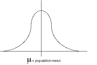
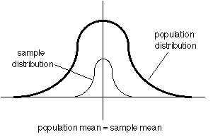
Graphically, this relationship can be expressed with the normal distribution, illustrating the grand mean(which is also called the population mean).and within the normal distribution we have smaller sub-distributions (Figure 1, below)


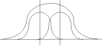
Under the experimental design, the researcher is evaluating the spread of the smaller distributions within the larger distribution. That is, under an experimental design, if the treatment effect was successful then one of these smaller distributions would be lying farther away from the other distributions and the grand mean (Figure 3, below).

NOTICE: The assumption of the research design is that all the sub-distributions have the same shape and that the researcher is testing thedifference between the location of the smaller distributions relative to the larger distributions.
Therefore, in making the assumption that all of the shapes of the distributions are equal we are saying that all of the within group variances are equal.
That is, group 1 (which is comprised of individuals which are randomly selected and randomly allocated to the group) has the same distribution shape as group 2 (which is comprised of individuals which are randomly selected and randomly allocated to the group), and group 3 (which is comprised of individuals which are randomly selected and randomly allocated to the group) and . . . .
This assumption is referred to as the homogeneity of variance assumption. Once the homogeneity of variance assumption is established then the researcher can more clearly evaluate the treatment effect by comparing only the "between group variances" or the measures
of central tendancy between groups. (see Figure 3, above)
In an experiment the researcher evaluates the between group difference that might exist because of the treatment conditions, based on the assumption that the measurement error is minimized.

Using the student's t-test to evaluate the random selection of individuals from a population
Consider that you were told that the average age of first time mothers in Canada was 23 years of age. However, from your experience in primary healthcare you felt that first time mothers in your hospital seemed much younger. So you set out to test the null hypothesis that any random selection of first time mothers would have the same age, on average, as the Canadian average. You decided to collect the ages of the next 10 first time mothers that entered the hospital. The age data are listed here:
mom1 age = 16, mom2 age = 18, mom3 age = 17, mom4 age = 20, mom5 age = 21, mom6 age = 15, mom7 age = 19, mom8 age = 16, mom9 age = 17, mom10 age = 17
The null hypothesis that you are testing in this scenario is:
H0: average age of first time mothers observed in your sample = average age of first time mothers in Canada
Which you decide to evaluate using the Student's t-test.
Begin by entering the age of each mother in your sample into the following form and click the button labelled "Compute Average", located at the bottom of the form
Next click the button labelled "Difference scores", located at the bottom of the next form to compute the exact difference between each observed age that you entered, and the average age that was computed.
Next click the button labelled "Square difference scores", located at the top of this next form to compute the squared difference scores from the table above.
Scroll to the bottom of this form and click the button labelled "Sum Scores" to produce the sum of squares. The sum of squares is the numerator in your estimation of variance computation and is the essential step in proceeding to compute differences between groups of scores.
Next click the button labelled "Estimates of Variance", located below to compute the variance scores from the data above.
Notice, you will be able to differentiate the sample variance and the sample standard deviation scores from the estimated population variance and the population standard deviation scores in the table below.
| Sample Variance = | |
| Sample Standard Deviation = | |
| Population Variance = | |
| Population Standard Deviation = | |
| Sample Standard Error (SE) = | |
|
95% Confidence Interval = 1.96 * SE 1.96 * = +/- |
The following steps enable you to evaluate null hypothesis using the Student's t test. That is, you are able to test the null hypothesis of the sample mean against the population mean, or stated another way, is the sample mean the same as the population mean?”.
Under the concept of randomized representative sampling we should expect that the sample mean should be the same as the population mean; and in our scenario, we are expecting that the average age of first time mothers in our sample is equal to the average age of first time mothers across Canada. However, before we begin using the t-test we have to make an assumption that the true value of the population mean is unknown and that the sample we drew from the population is representative of this population. Therefore, since the sample is representative of the population, then all of the values associated with the sample should be the same as the population. In using the t-test we assume that the population mean has a value of 0 and a variance (standard deviation) of 1. So that when we are applying the t-test, we are comparing our observed sample mean against the expected population mean of 0 with variance of 1. In the following table we can evaluate our sample estimates to test this concept.
| Single sample t test | t = (sample mean - 0) / standard error |
To test the concept: “is the sample
mean the same as the population
mean?” , which
is a test of the null hypothesis
that Ho: sample mean = population mean,we simply compare the
t scoreobserved
in the table above against the “t score ” critical ,
which we take from
a “t table ” based on the degrees of freedom of N-1
for the single sample test.
The “t score ” critical value for this sample of ten
items, given a degrees of freedom = 9, at a probability level
of p<0.05 is 2.26. If the
“t score” observed is greater than the “t score ”
critical
then we reject the null hypothesis and state that the sample mean is significantly
different than the population mean.
However, what if you didn't know the critical value but you wanted to evaluate the null hypothesis that the sample mean was equal to the population mean. You can do this using the information that you gained by computing the 95% confidence interval. In your scenario you were told that the population mean was equal to 23 years of age. However, you computed the sample mean to be 17.6 with a 95% confidence interval to be 1.176. Therefore, the bandwidth within which the expected population mean should fall according to your sample and estimates is between 16.424 as a lower limit value and 18.776 as an upper limit value. Since the population mean of 23 does not lie within this range then you reject the null hypothesis and state that your sample is significantly different than the expected population value.
Computations for Student's t-test are discussed in several texts including:
Hirsch, R.P., and Riegelman, R.K.,
Statistical First Aid: Interpretation of Health Research Data,
Boston, Blackwell Scientific Publications, page 73-75,1992.
Professor William J. Montelpare, Ph.D.,
Knapp R.G., and Miller, M.C., Clinical Epidemiology and Biostatistics ,
Baltimore, Williams and Wilkins, 1992.
 Click here to return to the Webulator Menu Page
Margaret and Wallace McCain Chair in Human Development and Health,
Department of Applied Human Sciences, Faculty of Science,
Health Sciences Building, University of Prince Edward Island,
550 Charlottetown, PE, Canada, C1A 4P3
(o) 902 620 5186
Visiting Professor, School of Healthcare, University of Leeds,
Leeds, UK, LS2 9JT
e-mail wmontelpare@upei.ca
Copyright © 2002--ongoing [University of Prince Edward Island]. All rights reserved.