
STATISTICAL APPLICATIONS FOR PATIENT ORIENTED PRIMARY HEALTHCARE RESEARCH
Explaining Pairwise Comparisons:
The purpose of the pairwise comparison t-test is to compare the average scores from two independent trials, for the same group of subjects.
For example, the pairwise comparison t-test would be useful to compare the average scores for a group of individuals tested on day 1 and then tested by the same procedure two weeks later. The assumption of the pairwise comparison t-test is that by using the same group of individuals, tested at two different times, the researcher will be able to maintain control over the homogeneity of variance within the sample group.
That is, when we computed the t-test for independent samples, as we did in our previous examples, a portion of the variability in the scores which comprised the mean for group1, and the mean for group2 was attributed to the intrinsic differences between the subjects which made up the two independent groups.
These potential differences are shown in the figure below.
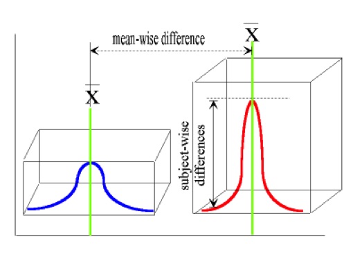
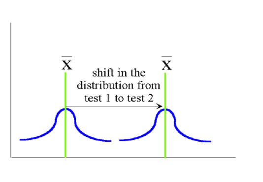
In the pairwise comparison t-test, the variability between the subjects is reduced by using the same subjects in two data collection sessions (for example, responses for a group of individuals are compared on a pre stimulus measure and a post stimulus measure). In the following diagram, the differences in mean scores are not attributed to differences in the variability of the subject from test1 to test2. Rather, the variability due to subjects is reduced by using the same individuals for the two test sessions. This technique is described as maintaining the homogeneity of variability due to sampling. As such, we are able to compare the shift in the distribution of scores from one sample time to another.
The null hypothesis for the paired or pairwise t-test is given below: H0: µ1 = µ2 or H0: µ1-µ2=0
An example:
Given that a group of 10 individuals agree to participate in a study of blood pressure changes following exposure to halogen lighting. In this experiment, a resting systolic blood pressure is recorded for each individual. The participants are then exposed to 20 minutes of halogen lighting by playing a video game in a room which is lit only by halogen lamps. A post exposure blood pressure reading is then recorded for each individual. The results are presented in the following data set.
The following is a stepwise procedure to compute the significance of the difference between the pre test blood pressures and the post test blood pressures. The statistical procedure will use the pairwise t-test approach.
| Participant Code | 001 | 002 | 003 | 004 | 005 | 006 | 007 | 008 | 009 | 010 |
| Pre test score | 34 | 54 | 60 | 68 | 53 | 70 | 81 | 87 | 65 | 55 |
| Post test score | 44 | 75 | 72 | 98 | 73 | 80 | 91 | 99 | 69 | 76 |
| Difference score | 10 | 21 | 12 | 30 | 20 | 10 | 10 | 12 | 4 | 21 |
Begin by entering the difference scores from the data from the following sample into the form and click the button labelled "Compute Average", located at the bottom of the form
Next we compute the differences between the mean score and each individual score by clicking the button labelled "compute", located at the bottom of the next form.
Next click the button labelled "Square Δ scores", located at the top of this next form to compute the squared difference scores from the table above.
Scroll to the bottom of this form and click the button labelled "Sum of Squares Scores" to produce the sum of squares. The sum of squares is the numerator in your estimation of variance computation and is the essential step in proceeding to compute differences between groups of scores.
Next click the button labelled "Estimates of Variance", located below to compute the variance scores from the data above.
Notice, you will be able to differentiate the sample variance and the sample standard deviation scores from the estimated population variance and the population standard deviation scores in the table below.
The following steps enable you to evaluate null hypothesis using the t-test. That is, you are able to test the null hypothesis of the sample mean against the population mean, or stated another way, is the sample mean for the set of difference scores the same as the population mean for the set of difference scores.
Under the concept of randomized representative sampling we should expect that the sample mean should be the same as the population mean; and in our scenario, we are expecting that the average difference score in our sample is equal to the average difference score for the population.
However, before we begin using the t-test we have to make an assumption that the true value of the population mean is unknown and that the sample we drew from the population is representative of this population. Therefore, since the sample is representative of the population, then all of the values associated with the sample should be the same as the population.
In using the t-test we assume that the population mean has a value of 0 and a variance (standard deviation) of 1. So that when we are applying the t-test, we are comparing our observed sample mean against the expected population mean of 0 with variance of 1. In the following table we can evaluate our sample estimates to test this concept.
To test the concept: “is the average difference score in the sample the same as the average difference score in the population ?” , which
is a test of the null hypothesis
that Ho: sample mean = population mean,we simply compare the
t scoreobserved
in the table above against the “t score ” critical ,
which we take from
a “t table ” based on the degrees of freedom of N-1
for the single sample test.
The “t score ” critical value for this sample of ten
items, given a degrees of freedom = 9, at a probability level
of p<0.05 is 2.26. If the
“t score” observed is greater than the “t score ”
critical
then we reject the null hypothesis and state that the sample mean is significantly
different than the population mean.
Computations for Pairwise t-tests are discussed in several texts including:
Hirsch, R.P., and Riegelman, R.K.,
Statistical First Aid: Interpretation of Health Research Data,
Boston, Blackwell Scientific Publications, page 73-75,1992.
Knapp R.G., and Miller, M.C., Clinical Epidemiology and Biostatistics ,
Baltimore, Williams and Wilkins, 1992.
 Click here to return to the Webulator Menu Page
Professor William J. Montelpare, Ph.D.,
Margaret and Wallace McCain Chair in Human Development and Health,
Department of Applied Human Sciences, Faculty of Science,
Health Sciences Building, University of Prince Edward Island,
550 Charlottetown, PE, Canada, C1A 4P3
(o) 902 620 5186
Visiting Professor, School of Healthcare, University of Leeds,
Leeds, UK, LS2 9JT
e-mail wmontelpare@upei.ca
Copyright © 2002--ongoing [University of Prince Edward Island]. All rights reserved.