Creating and Editing Delaunay Triangulations
The Delaunay triangulation is the most widely used triangulation in scientific computing. The properties associated with the triangulation provide a basis for solving a variety of geometric problems. The following examples demonstrate how to create, edit, and query Delaunay triangulations using the DelaunayTri class. Construction of constrained Delaunay triangulations is also demonstrated, together with an applications covering medial axis computation and mesh morphing.
Contents
- Example One: Create and Plot a 2D Delaunay Triangulation
- Example Two: Create and Plot a 3D Delaunay Triangulation
- Example Three: Access the Triangulation Data Structure
- Example Four: Edit a Delaunay Triangulation to Insert or Remove Points
- Example Five: Create a Constrained Delaunay Triangulation
- Example Six: Create a Constrained Delaunay Triangulation of a Geographical Map
- Example Seven: Curve Reconstruction from a Point Cloud
- Example Eight: Compute an Approximate Medial Axis of a Polygonal Domain
- Example Nine: Morph a 2D Mesh to a Modified Boundary
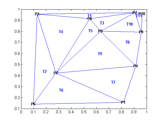
Example One: Create and Plot a 2D Delaunay Triangulation
This example shows you how to compute a 2D Delaunay triangulation and how to plot the triangulation together with the vertex and triangle labels.
x = rand(10,1);
y = rand(10,1);
dt = DelaunayTri(x,y)
dt =

  DelaunayTri

  Properties:
      Constraints: []
                X: [10x2 double]
    Triangulation: [11x3 double]
triplot(dt);
%
% Display the Vertex and Triangle labels on the plot
hold on
vxlabels = arrayfun(@(n) {sprintf('P%d', n)}, (1:10)');
Hpl = text(x, y, vxlabels, 'FontWeight', 'bold', 'HorizontalAlignment',...
           'center', 'BackgroundColor', 'none');
ic = incenters(dt);
numtri = size(dt,1);
trilabels = arrayfun(@(x) {sprintf('T%d', x)}, (1:numtri)');
Htl = text(ic(:,1), ic(:,2), trilabels, 'FontWeight', 'bold', ...
      'HorizontalAlignment', 'center', 'Color', 'blue');
hold off
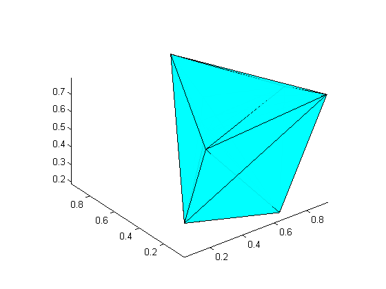
Example Two: Create and Plot a 3D Delaunay Triangulation
This example shows you how to compute a 3D Delaunay triangulation and how to plot the triangulation.
X = rand(10,3)
X =

    0.6557    0.7060    0.4387
    0.0357    0.0318    0.3816
    0.8491    0.2769    0.7655
    0.9340    0.0462    0.7952
    0.6787    0.0971    0.1869
    0.7577    0.8235    0.4898
    0.7431    0.6948    0.4456
    0.3922    0.3171    0.6463
    0.6555    0.9502    0.7094
    0.1712    0.0344    0.7547
dt = DelaunayTri(X)
dt =

  DelaunayTri

  Properties:
      Constraints: []
                X: [10x3 double]
    Triangulation: [22x4 double]
tetramesh(dt, 'FaceColor', 'cyan');
% To display large tetrahedral meshes use the convexHull method to
% compute the boundary triangulation and plot it using trisurf.
% For example;
% triboundary = convexHull(dt)
% trisurf(triboundary, X(:,1), X(:,2), X(:,3), 'FaceColor', 'cyan')
Example Three: Access the Triangulation Data Structure
There are two ways to access the triangulation data structure. One way is via the Triangulation property, the other way is using indexing.
Create a 2D Delaunay triangulation from 10 random points.
X = rand(10,2)
X =

    0.2760    0.7513
    0.6797    0.2551
    0.6551    0.5060
    0.1626    0.6991
    0.1190    0.8909
    0.4984    0.9593
    0.9597    0.5472
    0.3404    0.1386
    0.5853    0.1493
    0.2238    0.2575
dt = DelaunayTri(X)
dt =

  DelaunayTri

  Properties:
      Constraints: []
                X: [10x2 double]
    Triangulation: [12x3 double]
% The triangulation datastructure is;
dt.Triangulation
ans =

     4    10     1
     3     8     9
    10     4     5
     4     1     5
     1     6     5
     3    10     8
     1     3     6
     2     9     7
     6     3     7
     1    10     3
     3     2     7
     3     9     2
% Indexing is a shorthand way to query the triangulation. The format is
% dt(i, j) where j is the j'th vertex of the i'th triangle, standard
% indexing rules apply.
% The triangulation datastructure is
dt(:,:)
ans =

     4    10     1
     3     8     9
    10     4     5
     4     1     5
     1     6     5
     3    10     8
     1     3     6
     2     9     7
     6     3     7
     1    10     3
     3     2     7
     3     9     2
The second triangle is;
dt(2,:)
ans =

     3     8     9
The third vertex of the second triangle is;
dt(2,3)
ans =

     9
The first three triangles;
dt(1:3,:)
ans =

     4    10     1
     3     8     9
    10     4     5
Example Four: Edit a Delaunay Triangulation to Insert or Remove Points
This example shows you how to use index-based subscripting to insert or remove points. It is more efficient to edit a DelaunayTri to make minor modifications as opposed to recreating a new DelaunayTri from scratch, this is especially true if the dataset is large.
% Construct a Delaunay triangulation from
% 10 random points within a unit square
x = rand(10,1);
y = rand(10,1);
dt = DelaunayTri(x,y)
dt =

  DelaunayTri

  Properties:
      Constraints: []
                X: [10x2 double]
    Triangulation: [12x3 double]
% Insert 5 additional random points
dt.X(end+(1:5),:) = rand(5,2)
dt =

  DelaunayTri

  Properties:
      Constraints: []
                X: [15x2 double]
    Triangulation: [21x3 double]
Replace the fifth point
dt.X(5,:) = [0, 0]
dt =

  DelaunayTri

  Properties:
      Constraints: []
                X: [15x2 double]
    Triangulation: [21x3 double]
Remove the fourth point
dt.X(4,:) = []
dt =

  DelaunayTri

  Properties:
      Constraints: []
                X: [14x2 double]
    Triangulation: [19x3 double]
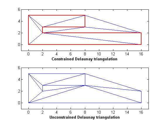
Example Five: Create a Constrained Delaunay Triangulation
This example shows you how to create a simple constrained Delaunay triangulation and illustrates the effect of the constraints.
X = [0 0; 16 0; 16 2; 2 2; 2 3; 8 3; 8 5; 0 5];
C = [1 2; 2 3; 3 4; 4 5; 5 6; 6 7; 7 8; 8 1];
dt = DelaunayTri(X, C);
subplot(2,1,1);
triplot(dt);
axis([-1 17 -1 6]);
xlabel('Constrained Delaunay triangulation', 'fontweight','b');
% Plot the constrained edges in red
hold on;
plot(X(C'),X(C'+size(X,1)),'-r', 'LineWidth', 2);
hold off;

% Now delete the constraints and plot the unconstrained Delaunay
dt.Constraints = [];
subplot(2,1,2);
triplot(dt);
axis([-1 17 -1 6]);
xlabel('Unconstrained Delaunay triangulation', 'fontweight','b');
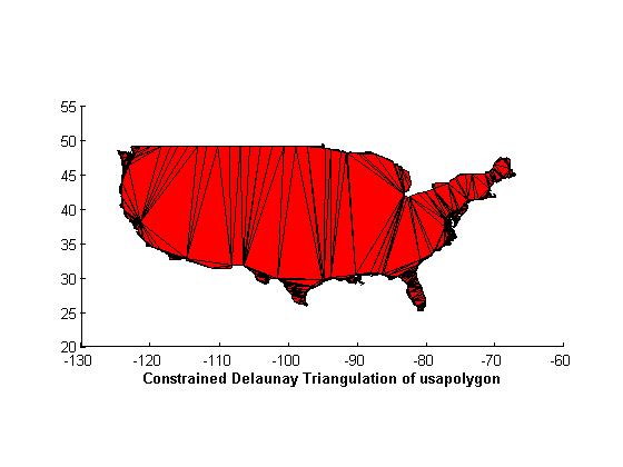
Example Six: Create a Constrained Delaunay Triangulation of a Geographical Map
Load a map of the perimeter of the conterminous United States. Construct a constrained Delaunay triangulation representing the polygon. This triangulation spans a domain that is bounded by the convex hull of the set of points. Filter out the triangles that are within the domain of the polygon and plot them. Note: The dataset contains duplicate datapoints; that is two or more datapoints have the same location. The duplicate points are rejected and the DelaunayTri reformats the constraints accordingly.
clf
load usapolygon
% Define an edge constraint between two successive
% points that make up the polygonal boundary.
nump = numel(uslon);
C = [(1:(nump-1))' (2:nump)'; nump 1];
dt = DelaunayTri(uslon, uslat, C);
io = dt.inOutStatus();
patch('faces',dt(io,:), 'vertices', dt.X, 'FaceColor','r');
axis equal;
axis([-130 -60 20 55]);
xlabel('Constrained Delaunay Triangulation of usapolygon', 'fontweight','b');
Warning: Duplicate data points have been detected and removed.
 The Triangulation indices and Constraints are defined with
 respect to the unique set of points in DelaunayTri property X.
Warning: Intersecting edge constraints have been split, this may have added
new points into the triangulation.
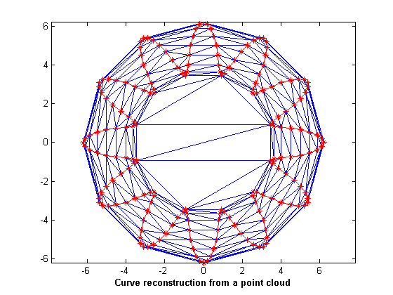
Example Seven: Curve Reconstruction from a Point Cloud
This example highlights the use of a Delaunay triangulation to reconstruct a polygonal boundary from a cloud of points. The reconstruction is based on the elegant Crust algorithm.
Reference: N. Amenta, M. Bern, and D. Eppstein. The crust and the beta-skeleton: combinatorial curve reconstruction. Graphical Models and Image Processing, 60:125-135, 1998.
% Create a set of points representing the point cloud
numpts=192;
t = linspace( -pi, pi, numpts+1 )';
t(end) = [];
r = 0.1 + 5*sqrt( cos( 6*t ).^2 + (0.7).^2 );
x = r.*cos(t);
y = r.*sin(t);
ri = randperm(numpts);
x = x(ri);
y = y(ri);
% Construct a Delaunay Triangulation of the point set.
dt = DelaunayTri(x,y);
tri = dt(:,:);
% Insert the location of the Voronoi vertices into the existing
% triangulation
V = dt.voronoiDiagram();
% Remove the infinite vertex
V(1,:) = [];
numv = size(V,1);
dt.X(end+(1:numv),:) = V;
Warning: Duplicate data points have been detected and removed.
 The Triangulation indices are defined with respect to
 the unique set of points in DelaunayTri property X.
% The Delaunay edges that connect pairs of sample points represent the
% boundary.
delEdges = dt.edges();
validx = delEdges(:,1) <= numpts;
validy = delEdges(:,2) <= numpts;
boundaryEdges = delEdges((validx & validy), :)';
xb = x(boundaryEdges);
yb = y(boundaryEdges);
clf;
triplot(tri,x,y);
axis equal;
hold on;
plot(x,y,'*r');
plot(xb,yb, '-r');
xlabel('Curve reconstruction from a point cloud', 'fontweight','b');
hold off;
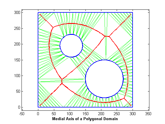
Example Eight: Compute an Approximate Medial Axis of a Polygonal Domain
This example demonstrates the creation of an approximate Medial Axis of a polygonal domain using a constrained Delaunay triangulation. The Medial Axis of a polygon is defined by the locus of the center of a maximal disk within the polygon interior.
% Construct a constrained Delaunay triangulation of a sample of points
% on the domain boundary.
load trimesh2d
dt = DelaunayTri(x,y,Constraints);
inside = dt.inOutStatus();
% Construct a TriRep to represent the domain triangles.
tr = TriRep(dt(inside, :), dt.X);

% Construct a set of edges that join the circumcenters of neighboring
% triangles; the additional logic constructs a unique set of such edges.
numt = size(tr,1);
T = (1:numt)';
neigh = tr.neighbors();
cc = tr.circumcenters();
xcc = cc(:,1);
ycc = cc(:,2);
idx1 = T < neigh(:,1);
idx2 = T < neigh(:,2);
idx3 = T < neigh(:,3);
neigh = [T(idx1) neigh(idx1,1); T(idx2) neigh(idx2,2); T(idx3) neigh(idx3,3)]';
% Plot the domain triangles in green, the domain boundary in blue and the
% medial axis in red.
clf;
triplot(tr, 'g');
hold on;
plot(xcc(neigh), ycc(neigh), '-r', 'LineWidth', 1.5);
axis([-10 310 -10 310]);
axis equal;
plot(x(Constraints'),y(Constraints'), '-b', 'LineWidth', 1.5);
xlabel('Medial Axis of a Polygonal Domain', 'fontweight','b');
hold off;
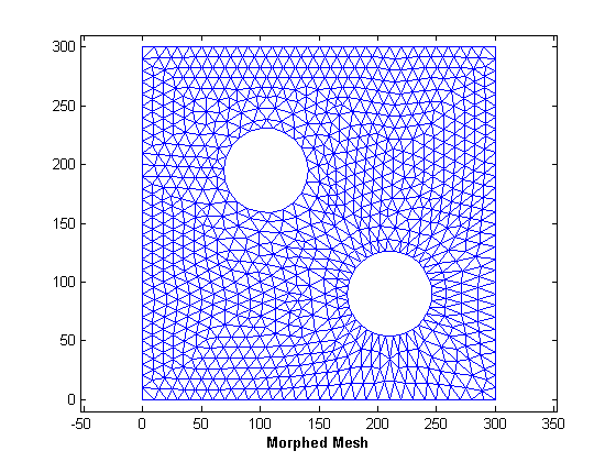
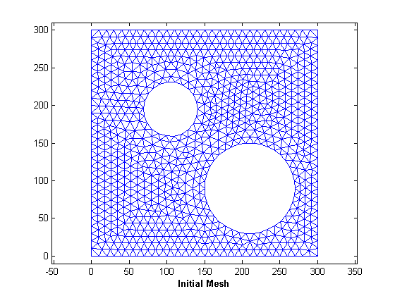
Example Nine: Morph a 2D Mesh to a Modified Boundary
This example shows how to morph a mesh of a 2D domain to accommodate a modification to the domain boundary.
Step 1: Load the data. The mesh to be morphed is defined by trife, xfe, yfe, which is a triangulation in face-vertex format.
load trimesh2d
clf; triplot(trife,xfe,yfe); axis equal;
axis([-10 310 -10 310]);
axis equal;
xlabel('Initial Mesh', 'fontweight','b');
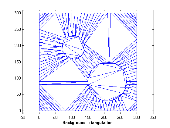
Step 2: Construct a background triangulation - a Constrained Delaunay triangulation of the set of points representing the mesh boundary. For each vertex of the mesh, compute a descriptor that defines it's location with respect to the background triangulation. The descriptor is the enclosing triangle together with the barycentric coordinates with respect to that triangle.
dt = DelaunayTri(x,y,Constraints);
clf; triplot(dt); axis equal;
axis([-10 310 -10 310]);
axis equal;
xlabel('Background Triangulation', 'fontweight','b');
descriptors.tri = dt.pointLocation(xfe, yfe);
descriptors.baryCoords = dt.cartToBary(descriptors.tri, [xfe yfe]);
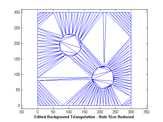
Step 3: Edit the background triangulation to incorporate the desired modification to the domain boundary.
cc1 = [210 90];
circ1 = (143:180)';
x(circ1) = (x(circ1)-cc1(1))*0.6 + cc1(1);
y(circ1) = (y(circ1)-cc1(2))*0.6 + cc1(2);
tr = TriRep(dt(:,:),x,y);
clf; triplot(tr); axis([-10 310 -10 310]); axis equal;
xlabel('Edited Background Triangulation - Hole Size Reduced', 'fontweight','b');
Step 4: Convert the descriptors back to Cartesian coordinates using the deformed background triangulation as a basis for evaluation.
Xnew = tr.baryToCart(descriptors.tri, descriptors.baryCoords);
tr = TriRep(trife, Xnew);
clf; triplot(tr);
axis([-10 310 -10 310]);
axis equal;
xlabel('Morphed Mesh', 'fontweight','b');