Grid-based Interpolation
A grid is a common and useful way to organize data. This data format represents values or intensities at discrete grid point locations. Grid-based data also fits naturally within the array-based environment MATLAB® provides.
When we work with gridded data we often need to know the values at locations other than at the grid points. Typically, we may need to refine the grid to improve resolution or de-refine the grid if it contains more detail than we practically need. Grid-based interpolation provides the functionality needed to carry out these tasks.
MATLAB provides the INTERP family of functions to support interpolation on grids that are in NDGRID or MESHGRID format. The griddedInterpolant class provides similar capabilities. It is designed to support the interpolation of grids in NDGRID format and leverage memory and performance advantages where possible. These improvements are readily apparent when interpolating the same grid in a repeated manner. In this scenario the overhead is accumulative. The griddedInterpolant can generally outperform the INTERP1/2/3/N functions as it is able to cache and reuse the same interpolating function.
The following examples demonstrate how to create a griddedInterpolant and how to use it effectively to perform grid-based interpolation.
Contents
- Refining a Coarse Grid
- Querying the Interpolant
- Selecting a Different Interpolation Method
- Interpolating Data in MESHGRID Format
- Interpolating Grids in General Dimensions
- Interpolating Grids that have Multiple Values at Each Gridpoint
- Interpolating Large Data Sets
- Interpolating a Dataset in a Repeated Manner
Refining a Coarse Grid
This example shows you how to create a griddedInterpolant for a gridded data set and then interpolate over a finer grid. We will begin by defining a function that generates values for X and Y input:
generatevalues = @(X,Y)(3*(1-X).^2.*exp(-(X.^2) - (Y+1).^2) ...
   - 10*(X/5 - X.^3 - Y.^5).*exp(-X.^2-Y.^2) ...
   - 1/3*exp(-(X+1).^2 - Y.^2));
We can create a 2D grid and then pass it to the generatevalues function to produce values at the grid points. The grid is created from a pair of grid vectors as follows:
xgv = -1.5:0.25:1.5;
ygv = -3:0.5:3;
[X,Y] = ndgrid(xgv,ygv);
Now generate the value data:
V = generatevalues(X,Y);
We can create an interpolant for this data set that supports interpolation within the grid. Since the interpolant behaves like a function we will give it the variable name F. The 'cubic' option specifies cubic interpolation.
F = griddedInterpolant(X, Y, V, 'cubic')
F =

  griddedInterpolant

  Properties:
    GridVectors: {2x1 cell}
         Values: [13x13 double]
         Method: 'cubic'
The interpolant F has 3 properties: The GridVectors are actually the vectors xgv and ygv we used to create the grid. The interpolant stores the grid in the compact form of GridVectors. This can save memory if the grid is large. GridVectors is a cell array so we can query the contents as follows:
gridvectorprop = F.GridVectors
firstgridvector = F.GridVectors{1}
secondgridvector = F.GridVectors{2}
gridvectorprop =

    [1x13 double]
    [1x13 double]


firstgridvector =

  Columns 1 through 7

   -1.5000   -1.2500   -1.0000   -0.7500   -0.5000   -0.2500         0

  Columns 8 through 13

    0.2500    0.5000    0.7500    1.0000    1.2500    1.5000


secondgridvector =

  Columns 1 through 7

   -3.0000   -2.5000   -2.0000   -1.5000   -1.0000   -0.5000         0

  Columns 8 through 13

    0.5000    1.0000    1.5000    2.0000    2.5000    3.0000
The values at the grid points are stored in the Values array. You can access the values using standard MATLAB syntax to index into the data. For example to inspect a 4-by-5 interval:
first4x5values = F.Values(1:4, 1:5)
first4x5values =

    0.0042    0.0028    0.0452    0.3265    0.3007
   -0.0050   -0.0671   -0.1285    0.3923    0.9838
   -0.0299   -0.2346   -0.5921    0.1483    1.8559
   -0.0752   -0.5260   -1.4478   -0.6798    2.4537
The interpolation technique is represented by the Method property. We selected cubic interpolation and our choice is reflected as follows:
theinterpolationmethod = F.Method
theinterpolationmethod =

cubic
We can now create a finer grid and use the interpolant to compute the values at these points. We will call these points the query points (Xq, Yq) to distinguish them from our original sample points.
xqgv = -1.5:0.1:1.5;
yqgv = -3:0.1:3;
[Xq,Yq] = ndgrid(xqgv,yqgv);
We can now evaluate over the refined grid to compute the corresponding values Vq at (Xq, Yq). Since we named our interpolant F, the calling syntax is
Vq = F(Xq, Yq);
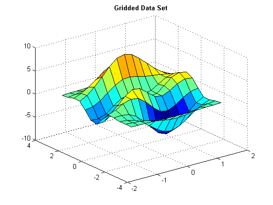
We can now generate a plot for comparison with our initial coarse plot.
figure
surf(X,Y,V)
title('Gridded Data Set', 'fontweight','b');

figure
surf(Xq, Yq, Vq);
title('Gridded Data Set Refined using Cubic Interpolation', 'fontweight','b');


Querying the Interpolant
We can query the interpolant at any location within the domain of the grid.
F(0.9,2.0)
ans =

    2.6536
You can compare this interpolated value with the value generated by the analytical expression.
generatevalues(0.9,2.0)
ans =

    2.6519
You can query the interpolant using an array of query points as opposed to arrays of query coordinates. We can demonstrate this by querying at random locations within the grid.
Xq =  -1.5 + 3.*rand(5,2);
Vq = F(Xq)
Vq =

   -1.7032
    2.0861
   -2.5200
    2.1331
    6.3799
Or using alternative syntax:
Vq = F(Xq(:,1), Xq(:,2))
Vq =

   -1.7032
    2.0861
   -2.5200
    2.1331
    6.3799
The interpolant supports queries within the domain of the grid. If your query point lies outside the domain of the grid the interpolant will return a NaN.
F(4,5)
ans =

   NaN
Selecting a Different Interpolation Method
You can change the interpolation method on-the-fly. For example, if you wish to use a spline method as opposed to cubic you can change it as follows:
F.Method = 'spline'
F =

  griddedInterpolant

  Properties:
    GridVectors: {2x1 cell}
         Values: [13x13 double]
         Method: 'spline'
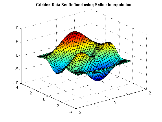
We can reevaluate and plot using the spline interpolation method.
xqgv = -1.5:0.1:1.5;
yqgv = -3:0.1:3;
[Xq,Yq] = ndgrid(xqgv,yqgv);
Vq = F(Xq, Yq);
We can now generate a plot for comparison with our initial coarse plot.
figure
surf(X,Y,V)
title('Gridded Data Set', 'fontweight','b');

figure
surf(Xq, Yq, Vq);
title('Gridded Data Set Refined using Spline Interpolation', 'fontweight','b');
Interpolating Data in MESHGRID Format
The griddedInterpolant class is designed to work with gridded data that conforms to the NDGRID format. This provides support for grids in general N-dimensions, including 1-D which can be regarded as a degenerate grid. In contrast, the MESHGRID format can only support grids in 2D and 3D. Both grid types have identical grid point coordinates; the difference is the format of the coordinate arrays.
If you wish to create a griddedInterpolant using MESHGRID data, you will need to convert the data to NDGRID format. In 2D this involves transposing the arrays as the following example demonstrates.
xgv = -1.5:0.25:1.5;
ygv = -3:0.5:3;
[X,Y] = meshgrid(xgv,ygv);
V = generatevalues(X,Y);
To convert the data to NDGRID format apply a transpose
X = X';
Y = Y';
V = V';
We can now create the interpolant
F = griddedInterpolant(X, Y, V)
F =

  griddedInterpolant

  Properties:
    GridVectors: {2x1 cell}
         Values: [13x13 double]
         Method: 'linear'
Converting 3D MESHGRID data to NDGRID format involves transposing each page of the 3D arrays. This is achieved using the PERMUTE function to interchange the rows (dimension 1) and columns (dimension 2). Here's an example that shows you how:
gv = -3:3;
[X,Y,Z] = meshgrid(gv);
V = X.^2 + Y.^2 + Z.^2;

P = [2 1 3];
X = permute(X,P);
Y = permute(Y,P);
Z = permute(Z,P);
V = permute(V,P);
We can now create the interpolant
F = griddedInterpolant(X, Y, Z, V)
F =

  griddedInterpolant

  Properties:
    GridVectors: {3x1 cell}
         Values: [7x7x7 double]
         Method: 'linear'
Likewise, when querying the interpolant using a MESHGRID, improved performance can be achieved by converting to NDGRID format. For example, if we wish to query our interpolant F using a MESHGRID composed of query points (Xq, Yq, Zq), we could convert the data to NDGRID format as follows:
[Xq, Yq, Zq] = meshgrid(0:0.5:2);
Xq = permute(Xq,P);
Yq = permute(Yq,P);
Zq = permute(Zq,P);
(Xq, Yq, Zq) is now in NDGRID format and can be queried efficiently.
Vq = F(Xq,Yq,Zq);
Interpolating Grids in General Dimensions
The griddedInterpolant class is not restricted to 2 and 3 dimensions. You can create an interpolant for 1D, 4D or higher. In practice, the memory required to represent the data may be the limiting factor in higher dimensions. This restriction can impact use in relatively low dimensions, less than ten, depending on the number of grid points and available computing power. The following example illustrates 1D interpolation using the PCHIP interpolation method.
X = 1:6;
V = [16 18 21 17 15 12];
F = griddedInterpolant(X,V,'pchip')
F =

  griddedInterpolant

  Properties:
    GridVectors: {[1 2 3 4 5 6]}
         Values: [16 18 21 17 15 12]
         Method: 'pchip'
We can now evaluate the interpolant over a finer interval.
Xq = 1:0.05:6;
Vq = F(Xq);
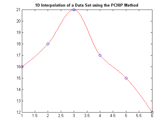
Plotting the query points in blue and the interpolated result in red we get:
plot(X,V,'ob',Xq,Vq,'-r')
title('1D Interpolation of a Data Set using the PCHIP Method', 'fontweight','b');
We can create and query a 4D interpolant as follows:
[X1, X2, X3, X4] = ndgrid(1:6);
V = X1.^2 + X2.^2 + X3.^2 + X4.^2;
F = griddedInterpolant(X1,X2,X3,X4,V)
F =

  griddedInterpolant

  Properties:
    GridVectors: {4x1 cell}
         Values: [4-D double]
         Method: 'linear'
Evaluation at a single 4D point
F(1.1,2.1,3.1,4.1)
ans =

   32.4000
Compare
(1.1)^2 + (2.1)^2 + (3.1)^2 + (4.1)^2
ans =

   32.0400
Evaluate at an array of 4D points
Xq = 1 + 5*rand(5,4);
Vq = F(Xq)
Vq =

   48.0991
   68.1209
  101.5174
   87.5036
   81.8984
Interpolating Grids that have Multiple Values at Each Gridpoint
In some applications there may be more than one value associated with each grid point and we may wish to interpolate each value set in turn. For example, if we have a grid representing the pixels in an image we may have three color intensities (RGB) associated with each grid point. There are two ways to interpolate this data. One approach is to create a separate interpolant for each of the three data sets. The other approach is to create a single interpolant and replace the values. The following example illustrates the replacement of values using a single interpolant.
xgv = -1.5:0.25:1.5;
ygv = -3:0.5:3;
[X,Y] = ndgrid(xgv,ygv);

% Create two distinct value sets for this grid

V1 = X.^3 - 3*(Y.^2);
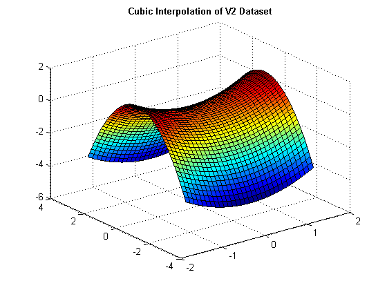
V2 = 0.5*(X.^2) - 0.5*(Y.^2);

% Now create an interpolant for the first value set
F = griddedInterpolant(X,Y,V1, 'cubic')
F =

  griddedInterpolant

  Properties:
    GridVectors: {2x1 cell}
         Values: [13x13 double]
         Method: 'cubic'
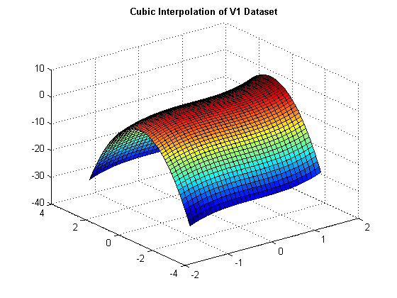
We can evaluate the V1 data set on a refined grid and plot the result
xqgv = -1.5:0.1:1.5;
yqgv = -3:0.1:3;
[Xq,Yq] = ndgrid(xqgv,yqgv);

Vq1 = F(Xq,Yq);
figure
surf(Xq,Yq,Vq1);
title('Cubic Interpolation of V1 Dataset', 'fontweight','b');
We can reuse the interpolant to interpolate the second dataset by replacing the Values data.
F.Values = V2
F =

  griddedInterpolant

  Properties:
    GridVectors: {2x1 cell}
         Values: [13x13 double]
         Method: 'cubic'
Vq2 = F(Xq,Yq);
figure
surf(Xq,Yq,Vq2);
title('Cubic Interpolation of V2 Dataset', 'fontweight','b');
Interpolating Large Data Sets
The griddedInterpolant class handles large data sets relatively efficiently. These data sets may consist of a grid of values generated externally and imported into MATLAB. For example, large 2D or 3D images scanned by an external source. In addition, such data sets may not have an explicitly defined grid of coordinate arrays. If the dataset is a large 3D image, the introduction of grid coordinate arrays would quadruple the memory.
The griddedInterpolant class allows you to create an interpolant from the grid of values and a default grid is then deduced from the size of the array. This default grid is defined in terms of grid vectors - a compact representation of the grid that uses very little memory.
To demonstrate this, we can use the PEAKS function to generate an array of values and then create an interpolant for this data set as follows:
V = peaks(10);
F = griddedInterpolant(V,'cubic')
F =

  griddedInterpolant

  Properties:
    GridVectors: {2x1 cell}
         Values: [10x10 double]
         Method: 'cubic'
Looking at the GridVectors property we can observe the vectors are deduced from the size of the V array. V is a 10x10 array and the corresponding grid vectors are 1:10 and 1:10
firstgridvector = F.GridVectors{1}
secondgridvector = F.GridVectors{2}
firstgridvector =

     1     2     3     4     5     6     7     8     9    10


secondgridvector =

     1     2     3     4     5     6     7     8     9    10
We can interpolate over a refined grid to improve resolution and fortunately we do not have to create a full grid to do so. We can evaluate using a pair of grid vectors and we package them within curly braces { } to communicate this intent. The default grid has a scaling of 1:10 so we will refine to pick up half intervals using 1:0.5:10. The corresponding query value Vq is as follows:
Vq = F({1:0.5:10, 1:0.5:10});
We can now plot the results side by side.
figure
surf(V);
title('Sample Values', 'fontweight','b');

figure
surf(Vq);
title('Cubic Interpolation using a Compact Grid', 'fontweight','b');
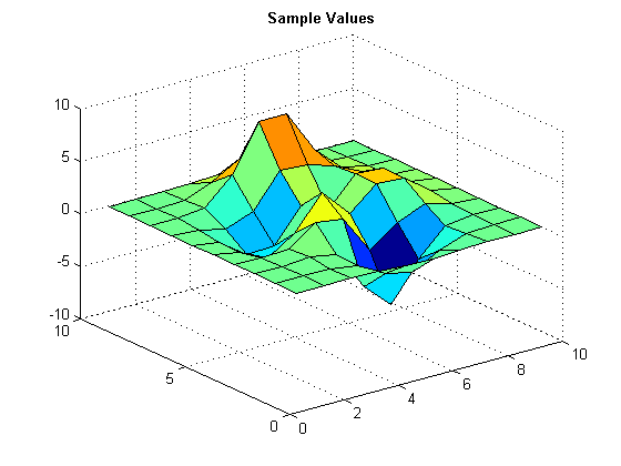
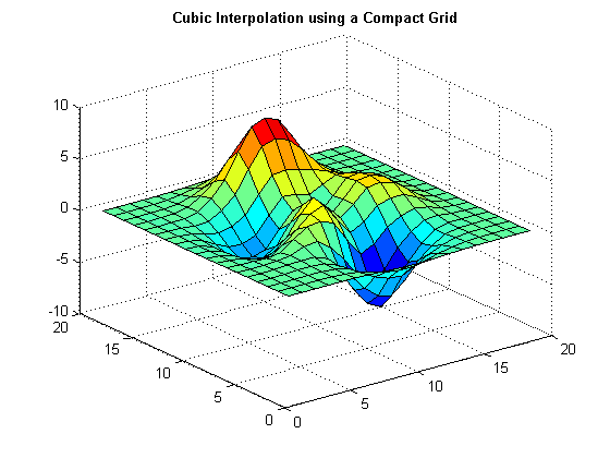
Note: When we plot the surface the SURF function also uses a default grid to produce the plot. In the first plot the values are represented by a 10-by-10 array and the second a 20-by-20. Hence the 0-to-10 and the 0-to-20 scales on the axes.
The Default Grid can be overridden by specifying grid vectors when you create the interpolant. For example, we could have constructed the interpolant as follows:
F = griddedInterpolant({10:19, 20:29}, V,'cubic')
F =

  griddedInterpolant

  Properties:
    GridVectors: {[10 11 12 13 14 15 16 17 18 19]  [1x10 double]}
         Values: [10x10 double]
         Method: 'cubic'
Evaluation would follow the same scaling
F(15,25)
ans =

   -0.0531
The default grid vectors could also have been replaced as follows:
F.GridVectors = {10:19, 20:29}
F =

  griddedInterpolant

  Properties:
    GridVectors: {[10 11 12 13 14 15 16 17 18 19]  [1x10 double]}
         Values: [10x10 double]
         Method: 'cubic'
Interpolating a Dataset in a Repeated Manner
In some applications it may be necessary to interpolate the same dataset in a repeated manner. The griddedInterpolant class can generally handle this scenario more efficiently than the INTERP functions. The griddedInterpolant class is able to reuse data computed during a previous query to speed up the computation of subsequent queries. The following example demonstrates this advantage:
Sample data set
[X, Y, Z] = ndgrid(1:100);
V = X.^2 + Y.^2 + Z.^2;
Performance data for INTERPN
tic;
for i = 1:1000
Xq = 100*rand();
Yq = 100*rand();
Zq = 100*rand();
Vq = interpn(X,Y,Z,V,Xq,Yq,Zq,'cubic');
end
interpnTiming = toc
interpnTiming =

   41.1202
Performance data for griddedInterpolant
tic;
F= griddedInterpolant(X,Y,Z,V, 'cubic');
for i = 1:1000
Xq = 100*rand();
Yq = 100*rand();
Zq = 100*rand();
Vq = F(Xq,Yq,Zq);
end
griddedInterpolantTiming = toc
griddedInterpolantTiming =

    0.1234